scikit-learn 에서 제공되는 decision tree 를 학습하면 각 branching 과정에 대한 정보가 모델에 저장됩니다. 이를 이용하면 tree traversal visualization 을 하거나, parameters 를 저장하여 직접 decsion rules based classifier 를 만들 수 있습니다. 이번 포스트에서는 학습된 decision tree 의 parameters 를 이용하는 방법을 소개합니다.
Brief review of decision tree
의사결정나무는 데이터의 공간을 직사각형으로 나눠가며 최대한 같은 종류의 데이터로 이뤄진 부분공간을 찾아가는 classifiers 입니다. 마치 clustering 처럼 비슷한 공간을 하나의 leaf node 로 나눠갑니다. 아래의 데이터를 분류하는 decision tree 를 학습한다고 가정합니다.

Decision tree 는 매번 각 변수에서 적절한 기준선을 찾아가며 공간을 이분 (bisect)합니다. 이 과정을 조건이 만족할 때까지 반복합니다.
위 그림처럼 tree 가 학습된 뒤, 우리는 각 공간에 대한 bisection path 를 얻을 수 있습니다. #0 공간인 root 는 #1 과 #2 로 나눠지고, #2 는 #3 과 #4 로 나눠집니다.
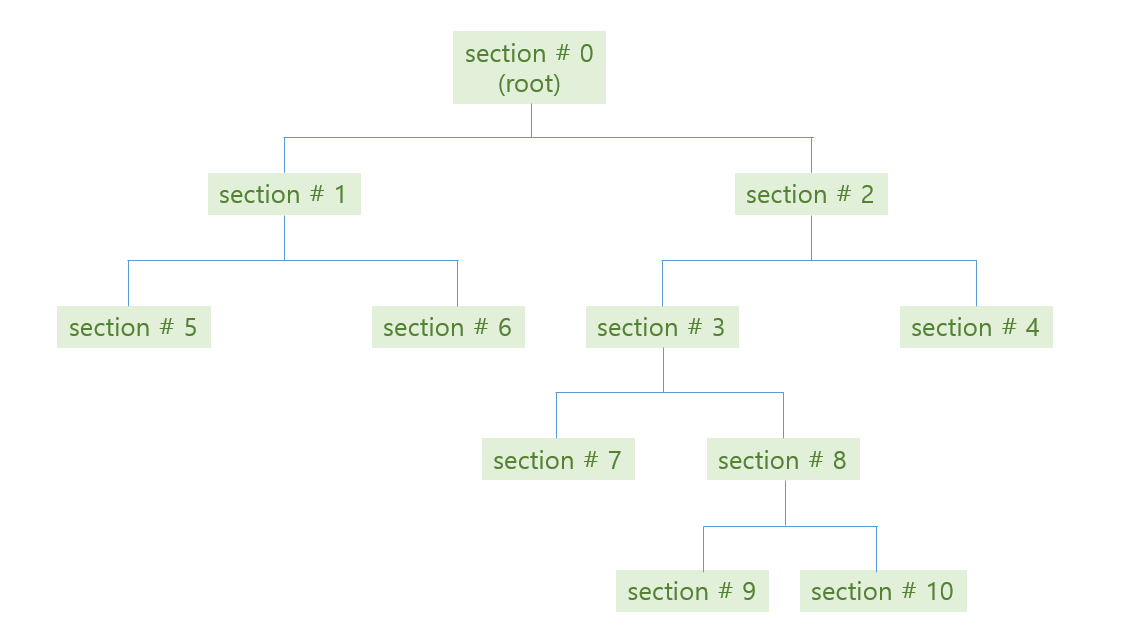
위 그림처럼 학습된 tree 의 각 decision rules 와 (parent, children) 의 관계는 아래와 같습니다.
| section no | # red | # blue | # entropy | # decision | # left child | # right child |
|---|---|---|---|---|---|---|
| 0 | 9 | 12 | 0.297 | \(x_1 \le 4\) | 1 | 2 |
| 1 | 3 | 6 | 0.276 | \(x_2 \le 7\) | 5 | 6 |
| 2 | 6 | 6 | 0.301 | \(x_2 \le 5\) | 3 | 4 |
| 3 | 6 | 2 | 0.244 | \(x_1 \le 8.5\) | 7 | 8 |
| 4 | 0 | 4 | 0 | - | - | - |
| 5 | 3 | 0 | 0 | - | - | - |
| 6 | 0 | 6 | 0 | - | - | - |
| 7 | 4 | 0 | 0 | - | - | - |
| 8 | 2 | 2 | 0.301 | \(x_2 \le 2.5\) | 9 | 10 |
| 9 | 0 | 2 | 0 | - | - | - |
| 10 | 2 | 0 | 0 | - | - | - |
이 정보를 이용하면 decision tree rules 를 시각화 하거나, 학습된 tree 의 parameters 를 다른 모델에 이식할 수 있습니다. 이번 포스트에서는 위 표의 정보들을 이용하여 text 로 된 tree traversal visualization 을 수행합니다.
Dataset
우리는 이전 포스트에서 만든 인공데이터를 이용하여 decision tree 가 학습한 tree path 의 parameters 를 이용하여 tree traversal 을 하겠습니다.
우리가 이용할 데이터는 아래처럼 만들 수 있습니다. 데이터 생성 함수는 이전 포스트를 참고하세요
from soydata.visualize import ipython_2d_scatter
from soydata.data import get_decision_tree_data_2

X_2, y_2 = get_decision_tree_data_2(n_samples=2000)
ipython_2d_scatter(X_2, y_2, marker_size=5, height=1000, width=1000, title='Synthetic dataset 2')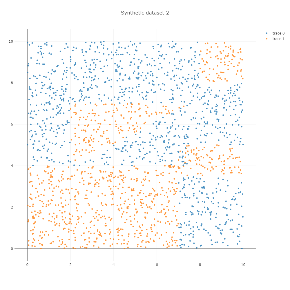
이를 학습하면 아래와 학습 과정을 얻을 수 있습니다. Decision tree 는 한 마디에서 하나의 변수만을 이용하기 때문에 사선의 경계면을 계단 형식의 경계선으로 학습합니다. Depth = 5 까지는 사각형의 모습을 하는데 이용되며, 그 이후 depth = 10 까지는 사선 방향의 경계면을 학습하는데 이용됩니다.
Parameters
우리의 목표는 brief review 에서의 표를 그릴 수 있는 정보를 얻는 것입니다.
각 마디의 children 구조는 tree_.children_left, tree_.children_right, tree_.threshold, tree_.feature 에 저장되어 있습니다. 마디의 개수는 총 59 개 입니다.
left = dt.tree_.children_left
right = dt.tree_.children_right
threshold = dt.tree_.threshold
features = dt.tree_.feature

print(left.shape) # (59,)
print(right.shape) # (59,)
print(threshold.shape) # (59,)
print(features.shape) # (59,)
각 마디의 idx 는 만들어진 순서대로입니다. Root node 는 left, right, threshold 등의 0 번째 입니다. left[0] = 1, right[0] = 6 은 root node 의 left child 은 1 번, right child 은 6 번 마디라는 의미입니다.
left 와 right children 을 살펴보면 - 값이 있습니다. 해당 마디가 leaf node 일 때 negative index 를 지닙니다.
print(left)
# array([ 1,  2, -1,  4, -1, -1,  7, -1,  9, 10, 11, 12, 13, -1, -1, -1, -1,
#        18, 19, 20, -1, 22, 23, -1, -1, -1, 27, 28, -1, 30, -1, -1, -1, 34,
#        35, 36, 37, -1, -1, -1, -1, 42, 43, 44, -1, -1, -1, 48, 49, -1, -1,
#        52, -1, -1, 55, -1, 57, -1, -1])

print(right)
# array([ 6,  3, -1,  5, -1, -1,  8, -1, 54, 17, 16, 15, 14, -1, -1, -1, -1,
#       33, 26, 21, -1, 25, 24, -1, -1, -1, 32, 29, -1, 31, -1, -1, -1, 41,
#       40, 39, 38, -1, -1, -1, -1, 47, 46, 45, -1, -1, -1, 51, 50, -1, -1,
#       53, -1, -1, 56, -1, 58, -1, -1])
비슷하게 features 도 negative value 를 지닙니다. 우리가 이용한 synthetic data 는 두 개의 변수로 이뤄져 있습니다. features[0] = 1 은 첫번째 decision 에 \(x_0, x_1\) 중 \(x_1\) 을 이용하였다는 의미입니다. index=2 는 leaf node 이기 때문에 decision 을 하지 않습니다. 그렇기 때문에 features[2] 에 negative index -2 가 저장되어 있습니다.
threshold 는 각 마디에서 이용된 threshold 입니다. features[0] 와 threshold[0] 를 합쳐 해석하면 is \(x_1 \le 4.00539017\) ? 입니다. Threshold 는 negative value 를 가질 수 있기 때문에, leaf nodes 를 확인하기 위해서는 children 이나 features 의 indices 를 살펴봐야 합니다.
print(features)
# array([ 1,  0, -2,  1, -2, -2,  0, -2,  1,  0,  1,  0,  1, -2, -2, -2, -2,
#         1,  0,  0, -2,  1,  0, -2, -2, -2,  0,  0, -2,  1, -2, -2, -2,  0,
#         1,  0,  1, -2, -2, -2, -2,  1,  1,  0, -2, -2, -2,  0,  0, -2, -2,
#         0, -2, -2,  0, -2,  1, -2, -2])

print(threshold)
# array([ 4.00539017,  7.00503731, -2.        ,  3.49398017, -2.        ,
#        -2.        ,  2.00174618, -2.        ,  6.98615742,  4.36656189,
#         4.98681259,  3.27961016,  4.26769447, -2.        , -2.        ,
#        -2.        , -2.        ,  4.8539381 ,  7.30683231,  6.99763584,
#        -2.        ,  4.68205166,  7.00949955, -2.        , -2.        ,
#        -2.        ,  7.4809618 ,  7.38458014, -2.        ,  4.61641979,
#        -2.        , -2.        , -2.        ,  5.66478252,  5.6269908 ,
#         4.47982836,  5.11054134, -2.        , -2.        , -2.        ,
#        -2.        ,  6.48954964,  5.00303268,  7.36141872, -2.        ,
#        -2.        , -2.        ,  7.06216717,  6.63848925, -2.        ,
#        -2.        ,  7.27605534, -2.        , -2.        ,  8.00331211,
#        -2.        ,  8.01910591, -2.        , -2.        ])
때로는 features 에 이름이 있기도 합니다. Visualization 을 위해서는 names 로 features 를 살펴봐도 좋습니다.
features = ['x{}'.format(feature) if feature >= 0 else None for feature in dt.tree_.feature]

print(features)
# ['x1', 'x0', None, 'x1', None, None, 'x0', None, 'x1', 'x0',
#  'x1', 'x0', 'x1', None, None, None, None, 'x1', 'x0', 'x0',
#   None, 'x1', 'x0', None, None, None, 'x0', 'x0', None, 'x1',
#   None, None, None, 'x0', 'x1', 'x0', 'x1', None, None, None,
#   None, 'x1', 'x1', 'x0', None, None, None, 'x0', 'x0', None,
#   None, 'x0', None, None, 'x0', None, 'x1', None, None]
각 마디에 포함되는 samples 의 개수는 value 에 저장되어 있습니다. 59 개 마디에 대하여 (1, n_classes) 의 array 형식입니다. value[0] 은 class 0 이 1045 개, class 1 이 961 개 포함되었다는 의미입니다. index=0 은 root node 이기 때문에 데이터셋 전체에 포함된 class 0, 1 의 개수가 각각 1045, 961 개 라는 의미입니다.
print(dt.tree_.value.shape)
# (59, 1, 2)

print(dt.tree_.value[0])
# array([[1045.,  961.]])
이를 이용하여 각 마디의 label 과 각 class 에 속할 확률을 만들 수 있습니다.
prob = np.asarray([freq/freq.sum() for freq in dt.tree_.value])
print(prob[0])
# array([[0.52093719, 0.47906281]])

labels = np.asarray([prob_.argmax() for prob_ in prob])
print(labels)
# array([0, 1, 1, 0, 0, 1, 0, 0, 0, 0, 1, 0, 1, 0, 1, 0, 1, 0, 1, 0, 0, 0,
#       0, 1, 0, 1, 1, 1, 1, 0, 0, 1, 1, 0, 1, 0, 0, 0, 1, 0, 1, 0, 0, 0,
#       0, 1, 0, 0, 1, 1, 1, 0, 0, 0, 0, 0, 1, 0, 1])
Tree traversal
이제 우리가 이용할 parameters 의 구조와 위치는 모두 파악했습니다. 이를 이용하여 tree traversal 을 수행합니다. \(i\) node 가 leaf 인지 확인하는 함수를 만듭니다.
def is_leaf(i):
    return features[i] is None
각 마디마다 children 이 있을 경우, right, left 순서로 children 에 관한 정보 (idx, depth, equation) 를 list 로 만듭니다. 이를 stack 에 쌓은 뒤 pop 을 할 것이기 때문에 right, left 순서로 만듭니다. Equation 은 \(x_1 \le 4.0095\) 와 같은 decision rule 입니다.
def make_stack_item(idx, depth):
    # (child idx, depth, equation)
    items = [
        (right[idx], depth, '{} > {}'.format(features[idx], '%.3f'%threshold[idx])),
        (left[idx], depth, '{} < {}'.format(features[idx], '%.3f'%threshold[idx]))
    ]
    return items
Print 를 할 때에는 depth 만큼의 indention 을 넣습니다. 각 마디의 label 과 데이터의 개수, 각 클래스에 속할 확률을 함께 출력햡니다.
def print_status(i, depth, equation):
    message = '{} ({}). label={} n_samples={}, prob=({})'.format(
        '|--- ' * depth, # indention
        equation,        # equation
        labels[i],       # label
        size[i],         # n samples
        ', '.join(['%.3f' % float(p) for p in prob[i][0]])) # prob
    print(message, flush=True)
Traversal 은 처음 root node 에 대하여 items 을 만든 뒤, stack 에 다른 마디가 없을 때까지 while loop 을 반복합니다.
Root node 의 children 을 이용하여 만든 두 개의 items 가 stack 에 포함되어 있습니다.
# initialize
stack = make_stack_item(idx=0, depth=1)
첫 번째 item 을 pop() 하면 left child 의 idx, depth, equation 이 return 됩니다.
while stack:
    idx, depth, equation = stack.pop()
이번 마디가 leaf node 이면 마디의 상태를 출력하고, children 을 지닌 branch 이면 자신의 상태를 출력한 뒤, 자신의 children 을 stack 에 쌓습니다. 이를 통하여 depth-first search 를 할 수 있습니다.
# if node is leaf print status
if is_leaf(idx):
    print_status(idx, depth, equation)
# else print status and add children (left, right) order
else:
    print_status(idx, depth, equation)
    stack += make_stack_item(idx, depth+1)
이 과정을 정리하면 아래와 같습니다.
def _print_tree_traversal(left, right, features, threshold, labels, size, prob):
    # initialize
    stack = make_stack_item(idx=0, depth=1)

    # print root
    print('Root n_samples={}, prob=({})'.format(
        size[0], ', '.join(['%.3f' % float(p) for p in prob[0][0]])))

    # while stack is not empty
    while stack:
        idx, depth, equation = stack.pop()
        # if node is leaf print status
        if is_leaf(idx):
            print_status(idx, depth, equation)
        # else print status and add children (left, right) order
        else:
            print_status(idx, depth, equation)
            stack += make_stack_item(idx, depth+1)
_print_tree_traversal() 함수는 decision tree 의 parameters 를 각각 입력받는 함수입니다. 학습된 decision tree 를 입력하면 이용가능한 형태의 parameters 를 만드는 함수를 하나 더 만들어줍니다. Features names 를 입력하면 이를 이용하고, 그렇지 않다면 \(x_0, x_1, \dots\) 처럼 변수 이름을 붙여줍니다.
def print_tree_traversal(dt, feature_names=None):

    left = dt.tree_.children_left
    right = dt.tree_.children_right
    threshold = dt.tree_.threshold

    if feature_names:
        features = [feature_names[f] if f >= 0 else None for f in dt.tree_.feature]
    else:
        features = ['x{}'.format(f) if f >= 0 else None for f in dt.tree_.feature]

    size = np.asarray([freq.sum() for freq in dt.tree_.value], dtype=np.int)
    prob = np.asarray([freq/freq.sum() for freq in dt.tree_.value])
    labels = np.asarray([prob_.argmax() for prob_ in prob])

    _print_tree_traversal(left, right, features, threshold, labels, size, prob)
print_tree_traversal() 를 실행한 결과입니다.
print_tree_traversal(dt)위 과정에 언급된 parameters 만을 저장하면 scikit-learn 을 이용하여 학습된 decision tree classifier 를 다른 언어로 구현할 수 있습니다.
Root n_samples=2006, prob=(0.521, 0.479)
|---  (x1 < 4.005). label=1 n_samples=824, prob=(0.220, 0.780)
|--- |---  (x0 < 7.005). label=1 n_samples=612, prob=(0.000, 1.000)
|--- |---  (x0 > 7.005). label=0 n_samples=212, prob=(0.854, 0.146)
|--- |--- |---  (x1 < 3.494). label=0 n_samples=181, prob=(1.000, 0.000)
|--- |--- |---  (x1 > 3.494). label=1 n_samples=31, prob=(0.000, 1.000)
|---  (x1 > 4.005). label=0 n_samples=1182, prob=(0.731, 0.269)
|--- |---  (x0 < 2.002). label=0 n_samples=229, prob=(1.000, 0.000)
|--- |---  (x0 > 2.002). label=0 n_samples=953, prob=(0.666, 0.334)
|--- |--- |---  (x1 < 6.986). label=0 n_samples=474, prob=(0.511, 0.489)
|--- |--- |--- |---  (x0 < 4.367). label=1 n_samples=135, prob=(0.141, 0.859)
|--- |--- |--- |--- |---  (x1 < 4.987). label=0 n_samples=31, prob=(0.613, 0.387)
|--- |--- |--- |--- |--- |---  (x0 < 3.280). label=1 n_samples=17, prob=(0.294, 0.706)
|--- |--- |--- |--- |--- |--- |---  (x1 < 4.268). label=0 n_samples=5, prob=(1.000, 0.000)
|--- |--- |--- |--- |--- |--- |---  (x1 > 4.268). label=1 n_samples=12, prob=(0.000, 1.000)
|--- |--- |--- |--- |--- |---  (x0 > 3.280). label=0 n_samples=14, prob=(1.000, 0.000)
|--- |--- |--- |--- |---  (x1 > 4.987). label=1 n_samples=104, prob=(0.000, 1.000)
|--- |--- |--- |---  (x0 > 4.367). label=0 n_samples=339, prob=(0.658, 0.342)
|--- |--- |--- |--- |---  (x1 < 4.854). label=1 n_samples=108, prob=(0.463, 0.537)
|--- |--- |--- |--- |--- |---  (x0 < 7.307). label=0 n_samples=50, prob=(0.960, 0.040)
|--- |--- |--- |--- |--- |--- |---  (x0 < 6.998). label=0 n_samples=39, prob=(1.000, 0.000)
|--- |--- |--- |--- |--- |--- |---  (x0 > 6.998). label=0 n_samples=11, prob=(0.818, 0.182)
|--- |--- |--- |--- |--- |--- |--- |---  (x1 < 4.682). label=0 n_samples=10, prob=(0.900, 0.100)
|--- |--- |--- |--- |--- |--- |--- |--- |---  (x0 < 7.009). label=1 n_samples=1, prob=(0.000, 1.000)
|--- |--- |--- |--- |--- |--- |--- |--- |---  (x0 > 7.009). label=0 n_samples=9, prob=(1.000, 0.000)
|--- |--- |--- |--- |--- |--- |--- |---  (x1 > 4.682). label=1 n_samples=1, prob=(0.000, 1.000)
|--- |--- |--- |--- |--- |---  (x0 > 7.307). label=1 n_samples=58, prob=(0.034, 0.966)
|--- |--- |--- |--- |--- |--- |---  (x0 < 7.481). label=1 n_samples=7, prob=(0.286, 0.714)
|--- |--- |--- |--- |--- |--- |--- |---  (x0 < 7.385). label=1 n_samples=4, prob=(0.000, 1.000)
|--- |--- |--- |--- |--- |--- |--- |---  (x0 > 7.385). label=0 n_samples=3, prob=(0.667, 0.333)
|--- |--- |--- |--- |--- |--- |--- |--- |---  (x1 < 4.616). label=0 n_samples=2, prob=(1.000, 0.000)
|--- |--- |--- |--- |--- |--- |--- |--- |---  (x1 > 4.616). label=1 n_samples=1, prob=(0.000, 1.000)
|--- |--- |--- |--- |--- |--- |---  (x0 > 7.481). label=1 n_samples=51, prob=(0.000, 1.000)
|--- |--- |--- |--- |---  (x1 > 4.854). label=0 n_samples=231, prob=(0.749, 0.251)
|--- |--- |--- |--- |--- |---  (x0 < 5.665). label=1 n_samples=57, prob=(0.333, 0.667)
|--- |--- |--- |--- |--- |--- |---  (x1 < 5.627). label=0 n_samples=20, prob=(0.950, 0.050)
|--- |--- |--- |--- |--- |--- |--- |---  (x0 < 4.480). label=0 n_samples=2, prob=(0.500, 0.500)
|--- |--- |--- |--- |--- |--- |--- |--- |---  (x1 < 5.111). label=0 n_samples=1, prob=(1.000, 0.000)
|--- |--- |--- |--- |--- |--- |--- |--- |---  (x1 > 5.111). label=1 n_samples=1, prob=(0.000, 1.000)
|--- |--- |--- |--- |--- |--- |--- |---  (x0 > 4.480). label=0 n_samples=18, prob=(1.000, 0.000)
|--- |--- |--- |--- |--- |--- |---  (x1 > 5.627). label=1 n_samples=37, prob=(0.000, 1.000)
|--- |--- |--- |--- |--- |---  (x0 > 5.665). label=0 n_samples=174, prob=(0.885, 0.115)
|--- |--- |--- |--- |--- |--- |---  (x1 < 6.490). label=0 n_samples=129, prob=(0.953, 0.047)
|--- |--- |--- |--- |--- |--- |--- |---  (x1 < 5.003). label=0 n_samples=15, prob=(0.600, 0.400)
|--- |--- |--- |--- |--- |--- |--- |--- |---  (x0 < 7.361). label=0 n_samples=9, prob=(1.000, 0.000)
|--- |--- |--- |--- |--- |--- |--- |--- |---  (x0 > 7.361). label=1 n_samples=6, prob=(0.000, 1.000)
|--- |--- |--- |--- |--- |--- |--- |---  (x1 > 5.003). label=0 n_samples=114, prob=(1.000, 0.000)
|--- |--- |--- |--- |--- |--- |---  (x1 > 6.490). label=0 n_samples=45, prob=(0.689, 0.311)
|--- |--- |--- |--- |--- |--- |--- |---  (x0 < 7.062). label=1 n_samples=14, prob=(0.071, 0.929)
|--- |--- |--- |--- |--- |--- |--- |--- |---  (x0 < 6.638). label=1 n_samples=11, prob=(0.000, 1.000)
|--- |--- |--- |--- |--- |--- |--- |--- |---  (x0 > 6.638). label=1 n_samples=3, prob=(0.333, 0.667)
|--- |--- |--- |--- |--- |--- |--- |---  (x0 > 7.062). label=0 n_samples=31, prob=(0.968, 0.032)
|--- |--- |--- |--- |--- |--- |--- |--- |---  (x0 < 7.276). label=0 n_samples=3, prob=(0.667, 0.333)
|--- |--- |--- |--- |--- |--- |--- |--- |---  (x0 > 7.276). label=0 n_samples=28, prob=(1.000, 0.000)
|--- |--- |---  (x1 > 6.986). label=0 n_samples=479, prob=(0.820, 0.180)
|--- |--- |--- |---  (x0 < 8.003). label=0 n_samples=349, prob=(1.000, 0.000)
|--- |--- |--- |---  (x0 > 8.003). label=1 n_samples=130, prob=(0.338, 0.662)
|--- |--- |--- |--- |---  (x1 < 8.019). label=0 n_samples=44, prob=(1.000, 0.000)
|--- |--- |--- |--- |---  (x1 > 8.019). label=1 n_samples=86, prob=(0.000, 1.000)
위 결과에서 살펴볼 수 있듯이 처음 \(x_1 < 4.005\) 를 통하여 아래 부분은 큰 어려움없이 분류가 잘 됩니다. 대부분의 depth 를 삼각형 모양의 경계면을 학습하는데 이용하고 있음을 확인할 수 있습니다.