Named Entity Recognition (NER) 은 문장에서 특정한 종류의 단어를 찾아내는 information extraction 문제 중 하나입니다. ‘디카프리오가 나온 영화 틀어줘’라는 문장에서 ‘디카프리오’를 사람으로 인식하는 것을 목표로 합니다. 단어열로 표현된 문장에 각 단어의 종류를 인식하는 sequential labeling 방법이 주로 이용되었습니다. 최근에는 Recurrent Neural Network 와 같은 방법도 이용되지만, 오래전부터 Conditional Random Field (CRF) 가 이용되었습니다. 특히 CRF 모델은 named entities 를 판별하는 규칙을 해석할 수 있다는 점에서 유용합니다. 이번 포스트에서는 CoNLL 2002 NER task dataset 에 CRF 를 적용하여 NER 모델을 만드는 과정에 대하여 설명합니다.
Conditional Random Field
Named Entity Recognition (NER) 을 위하여 전통적으로 많이 이용되는 모델은 Conditional Random Field (CRF) 입니다. 이번 포스트에서는 CRF 을 간단하게 정리하며 시작합니다. Potential functions 나 Maximum Entropy Markov Model (MEMM) 과의 차이는 이전 포스트를 보시기 바랍니다.
일반적으로 classification 이라 하면, 하나의 입력 벡터 \(x\) 에 대하여 하나의 label 값 \(y\) 를 return 하는 과정입니다. 그런데 입력되는 \(x\) 가 벡터가 아닌 sequence 일 경우가 있습니다. \(x\) 를 길이가 \(n\) 인 sequence, \(x = [x_1, x_2, \ldots, x_n]\) 라 할 때, 같은 길이의 \(y = [y_1, y_2, \ldots, y_n]\) 을 출력해야 하는 경우가 있습니다. Labeling 은 출력 가능한 label 중에서 적절한 것을 선택하는 것이기 때문에 classification 입니다. 데이터의 형식이 벡터가 아닌 sequence 이기 때문에 sequential data 에 대한 classification 이라는 의미로 sequential labeling 이라 부릅니다.
띄어쓰기 문제나 품사 판별이 대표적인 sequential labeling 입니다. 품사 판별은 주어진 단어열 \(x\) 에 대하여 품사열 \(y\) 를 출력합니다.
- \(x = [이것, 은, 예문, 이다]\) .
- \(y = [명사, 조사, 명사, 조사]\) .
띄어쓰기는 길이가 \(n\) 인 글자열에 대하여 [띈다, 안띈다] 중 하나로 이뤄진 Boolean sequence \(y\) 를 출력합니다.
- \(x = 이것은예문입니다\) .
- \(y = [0, 0, 1, 0, 1, 0, 0, 1]\) .
이 과정을 확률모형으로 표현하면 주어진 \(x\) 에 대하여 \(P(y \vert x)\) 가 가장 큰 \(y\) 를 찾는 문제입니다. 이를 아래처럼 기술하기도 합니다. \(x_{1:n}\) 은 길이가 \(n\) 인 sequence 라는 의미입니다.
\[argmax_y P(y_{1:n} \vert x_{1:n})\]CRF 는 이를 위하여 앞, 뒤 단어와 품사 정보들을 이용합니다. ‘너’라는 단어 앞, 뒤의 단어와 우리가 이미 예측한 앞 단어의 품사를 이용한다면 더 정확한 품사 판별을 할 수 있습니다. 특히 앞 단어의 품사를 이용하면 문법적인 비문을 방지할 수 있습니다. 예를 들어 ‘조사’ 다음에는 ‘조사’가 등장하기 어렵습니다. 앞에 조사가 등장하였다면, 이번 단어의 품사가 조사일 가능성은 낮도록 유도할 수 있습니다.
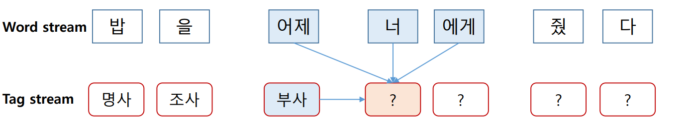
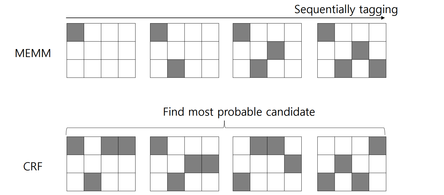
그런데 위의 그림처럼 작동하는 sequential labeling algorithm 은 Maximum Entropy Markov Model (MEMM) 입니다. MEMM 은 label bias 라는 문제가 발생하고, 이를 해결한 방법이 CRF 입니다. 단어열의 길이가 \(n\) 일 때, \(n\) 번의 classification 을 수행하지 않고, 전체적인 문맥을 고려하여 한 번의 classification 을 수행함으로써 label bias 문제를 해결합니다.
이 개념은 아래의 그림처럼 표현할 수도 있습니다. MEMM 은 입력된 sequence data \(x\) 에 대하여 앞부분부터 적절한 labels 을 찾아갑니다. 하지만 CRF 는 가능성이 있는 sequence \(y\) 후보를 몇 개 선택한 뒤, 가장 적합한 하나의 label 을 고릅니다.
CRF 를 이해하기 위해서는 반드시 potential function 을 이해해야 합니다. Potential function 은 \(n\) 개의 단어열을 각각 high dimensional sparse vector 로 표현하는 방법입니다. 일종의 Boolean filter 처럼 작동합니다. 아래의 예시는 [이것, 은, 예문, 이다] 라는 네 단어로 구성된 문장에 대하여 세 종류의 potential function 을 이용한 결과입니다. 길이가 4 인 문장은 4 by 3 Boolean matrix, \(x_{vec}\) 로 표현됩니다.
- \(x = [이것, 은, 예문, 이다]\) .
- \(F_1 = 1\) if \(x_{i-1} =\) ‘이것’ & \(x_i =\) ‘은’ else \(0\)
- \(F_2 = 1\) if \(x_{i-1} =\) ‘이것’ & \(x_i =\) ‘예문’ else \(0\)
- \(F_3 = 1\) if \(x_{i-1} =\) ‘은’ & \(x_i =\) ‘예문’ else \(0\)
- \(x_{vec} = [(0, 0, 0), (1, 0, 0), (0, 0, 1), (0, 0, 0)]\) .
문장이 \(x_{vec}\) 과 같은 vector 로 표현된 다음에는 logistic regression 이 적용됩니다. CRF 는 potential function 이 포함되어 있는 logistic regression 입니다. CRF 의 의 \(P(y_{1:n} \vert x_{1:n})\) 는 아래처럼 기술됩니다.
\[P(y \vert x) = \frac{exp(\sum_{j=1}^{m} \sum_{i=1}^{n} \lambda_j f_j (x, i, y_i, y_{i-1}))}{ \sum_{y^{`}} exp(\sum_{j^{`}=1}^{m} \sum_{i=1}^{n} \lambda_j f_j (x, i, y_i^{`}, y_{i-1}^{`})) }\]CoNLL 2002 dataset
CoNLL 2002 에서는 language independent 하게 적용할 수 있는 named entity recognition 방법을 연구하기 위하여 competition 을 열었습니다. 그리고 이 데이터는 Python NLP toolkit 인 nltk에 공개되어 있습니다. nltk 를 이용하여 다운로드 받을 수 있습니다.
nltk.corpus 에는 conll2002 가 있습니다. fields 를 살펴보면 esp. 와 ned. 가 있습니다. esp 는 스페인어 데이터이며, ned 는 네델란드어 데이터입니다. 각각 train 용과 test a, test b 용 데이터로 구성되어 있습니다.
import nltk

print(nltk.corpus.conll2002.fileids())
# ['esp.testa', 'esp.testb', 'esp.train', 'ned.testa', 'ned.testb', 'ned.train']
pip install 을 이용하여 nltk 를 설치하면 (pip install nltk) 처음에는 corpus 의 데이터들이 포함되어 있지 않습니다. 만약 위 코드에서 오류가 발생한다면 아래와 같이 특정 corpus 를 다운로드 할 수 있습니다.
nltk.download('conll2002')학습과 테스트용 데이터를 불러옵니다.
train_sents = list(nltk.corpus.conll2002.iob_sents('esp.train'))
test_sents = list(nltk.corpus.conll2002.iob_sents('esp.testb'))
train / test sentences 는 (단어, 품사, NER tag) 의 list 형식으로 구성되어 있습니다. 아래의 예시는 문장 “Melbourne(Australia), 25 may (EFE).”에 대하여 품사 판별이 된 데이터에 대한 B-I-O NER tag 입니다.
train_sents[0]
# [('Melbourne', 'NP', 'B-LOC'),
#  ('(', 'Fpa', 'O'),
#  ('Australia', 'NP', 'B-LOC'),
#  (')', 'Fpt', 'O'),
#  (',', 'Fc', 'O'),
#  ('25', 'Z', 'O'),
#  ('may', 'NC', 'O'),
#  ('(', 'Fpa', 'O'),
#  ('EFE', 'NC', 'B-ORG'),
#  (')', 'Fpt', 'O'),
#  ('.', 'Fp', 'O')]
B-I-O tag
B-I-O tag 는 NER 과 같은 information extraction 작업에 자주 이용되는 tagset 입니다. Named entity 는 두 개 이상의 단어의 합으로 만들어 질 수 있습니다. “Barack Obama” 처럼 두 개 이상의 단어로 이뤄진 person 을 표현하기 위하여 (Barack, B), (Obama, I) 처럼 태그를 부착합니다. B 는 begin 의 약자이며, I 는 inside, O 는 outside 의 약자입니다. Named entity 가 시작될 때 B 를 부여합니다. Named entity 가 아닌 단어들은 모두 O 를 부여합니다.
Competition 에서 제공하는 NER tasks 는 주로 Person, Location, Organization 을 인식하는 경우가 많습니다. 위의 CoNLL 2002 역시 그러하며, B-LOC 는 location 이 시작되는 지점이라는 의미입니다.
PyCRFSuite official tutorial
PyCRFSuite는 c++ 로 구현된 CRFSuite 구현체를 Python 환경에서 이용할 수 있도록 도와주는 라이브러리입니다. 우리는 이전에 이를 이용하여 한국어 띄어쓰기 교정기를 만들어 보았습니다.
PyCRFSuite 의 official tutorial 은 CoNLL2002 dataset 을 이용한 NER model 을 학습하는 것입니다. 이 포스트에서는 PyCRFSuite 의 official tutorial 내용 중 일부를 설명합니다. 그리고 다음 장에서 NER tasks 에서 중요한 정보가 무엇인지에 대하여 살펴봅니다.
PyCRFSuite 를 이용하기 위해서는 potential function 을 직접 디자인하여야 합니다. Official tutorial 의 word2features 는 문장 sent 의 시점 \(i\) 에 대한 potential function 입니다.
아래의 함수는 \(i\) 시점의 앞/뒤 단어인 \(i-1\), \(i+1\) 에 대하여 소문자화 한 단어, 각 단어의 뒤의 2, 3 글자 (latin 계열 단어에서는 suffix 가 유용한 힌트가 됩니다), 단어의 품사 등을 이용합니다.
def word2features(sent, i):
    word = sent[i][0]
    postag = sent[i][1]
    features = [
        'bias',
        'word.lower=' + word.lower(),
        'word[-3:]=' + word[-3:],
        'word[-2:]=' + word[-2:],
        'word.isupper=%s' % word.isupper(),
        'word.istitle=%s' % word.istitle(),
        'word.isdigit=%s' % word.isdigit(),
        'postag=' + postag,
        'postag[:2]=' + postag[:2],
    ]
    if i > 0:
        word1 = sent[i-1][0]
        postag1 = sent[i-1][1]
        features.extend([
            '-1:word.lower=' + word1.lower(),
            '-1:word.istitle=%s' % word1.istitle(),
            '-1:word.isupper=%s' % word1.isupper(),
            '-1:postag=' + postag1,
            '-1:postag[:2]=' + postag1[:2],
        ])
    else:
        features.append('BOS')

    if i < len(sent)-1:
        word1 = sent[i+1][0]
        postag1 = sent[i+1][1]
        features.extend([
            '+1:word.lower=' + word1.lower(),
            '+1:word.istitle=%s' % word1.istitle(),
            '+1:word.isupper=%s' % word1.isupper(),
            '+1:postag=' + postag1,
            '+1:postag[:2]=' + postag1[:2],
        ])
    else:
        features.append('EOS')

    return features
이를 정리하면 아래와 같습니다.
| Feature / position | \(i-1\) | \(i\) | \(i+1\) |
|---|---|---|---|
| bias | o | ||
| word lower | o | o | o |
| word[-3:] | o | ||
| word[-2:] | o | ||
| word is upper? | o | o | o |
| word is title? | o | o | o |
| word is digit? | o | ||
| postag | o | o | o |
| postag[:2] | o | o | o |
그 외 문장을 potential functions 이 적용된 sparse vector 열로 변환하거나 문장에서 단어, NER tags 를 가져오는 함수들은 아래와 같습니다.
def sent2features(sent):
    return [word2features(sent, i) for i in range(len(sent))]

def sent2labels(sent):
    return [label for token, postag, label in sent]

def sent2tokens(sent):
    return [token for token, postag, label in sent]
학습 데이터의 첫 문장, 첫 단어의 featuers 는 아래와 같습니다. 꾀 많은 정보를 이용합니다.
sent2features(train_sents[0])[0]
# ['bias',
#  'word.lower=melbourne',
#  'word[-3:]=rne',
#  'word[-2:]=ne',
#  'word.isupper=False',
#  'word.istitle=True',
#  'word.isdigit=False',
#  'postag=NP',
#  'postag[:2]=NP',
#  'BOS',
#  '+1:word.lower=(',
#  '+1:word.istitle=False',
#  '+1:word.isupper=False',
#  '+1:postag=Fpa',
#  '+1:postag[:2]=Fp']
이를 이용하여 문장을 학습 가능한 형태의 데이터로 변환합니다.
X_train = [sent2features(s) for s in train_sents]
y_train = [sent2labels(s) for s in train_sents]

X_test = [sent2features(s) for s in test_sents]
y_test = [sent2labels(s) for s in test_sents]
모델에 데이터를 append 하여 학습할 준비를 합니다.
import pycrfsuite
trainer = pycrfsuite.Trainer(verbose=False)

for xseq, yseq in zip(X_train, y_train):
    trainer.append(xseq, yseq)
PyCRFSuite 의 parameter setting 을 합니다. Official tutorial 과 다른 세팅을 하나 추가하였습니다. Official tutorial 에서는 feature 의 minimum frequency 를 1로 이용합니다. 한 번만 등장한 feature 라도 학습에 이용한다는 의미인데, 이는 over-fitting 을 야기하기도 하며, 모델의 크기를 지나치게 크게 키웁니다.
이를 방지하기 위하여 ‘feature.minfreq’: 5 로 설정하여 최소 5 번 이상 등장한 features 만 이용하도록 설정합니다.
import pycrfsuite
trainer.set_params({
    'c1': 1.0,   # coefficient for L1 penalty
    'c2': 1e-3,  # coefficient for L2 penalty
    'max_iterations': 50,  # stop earlier

    # include transitions that are possible, but not observed
    'feature.possible_transitions': True,

    # minimum frequency
    'feature.minfreq': 5
})
모델을 학습한 뒤, 학습된 모델을 tagger 로 불러들입니다.
trainer.train('conll2002-esp.crfsuite')
tagger = pycrfsuite.Tagger()
tagger.open('conll2002-esp.crfsuite')
테스트 문장에 대하여 NER tagging 을 수행하여 학습 여부를 확인합니다.
example_sent = test_sents[0]
print(' '.join(sent2tokens(example_sent)), end='\n\n')

print("Predicted:", ', '.join(tagger.tag(sent2features(example_sent))))
print("Correct:  ", ', '.join(sent2labels(example_sent)))
결과는 아래와 같습니다.
La Coruña , 23 may ( EFECOM ) .

Predicted: B-LOC, I-LOC, O, O, O, O, B-ORG, O, O
Correct:   B-LOC, I-LOC, O, O, O, O, B-ORG, O, O
Official tutorial 에서는 scikit learn 의 classification_report 를 이용하여 tagging performance 를 보여주는 함수를 제공합니다.
from sklearn.metrics import classification_report, confusion_matrix

def bio_classification_report(y_true, y_pred):
    """
    Classification report for a list of BIO-encoded sequences.
    It computes token-level metrics and discards "O" labels.

    Note that it requires scikit-learn 0.15+ (or a version from github master)
    to calculate averages properly!
    """
    lb = LabelBinarizer()
    y_true_combined = lb.fit_transform(list(chain.from_iterable(y_true)))
    y_pred_combined = lb.transform(list(chain.from_iterable(y_pred)))

    tagset = set(lb.classes_) - {'O'}
    tagset = sorted(tagset, key=lambda tag: tag.split('-', 1)[::-1])
    class_indices = {cls: idx for idx, cls in enumerate(lb.classes_)}

    return classification_report(
        y_true_combined,
        y_pred_combined,
        labels = [class_indices[cls] for cls in tagset],
        target_names = tagset,
    )
이를 이용하여 학습된 모델의 성능을 확인합니다.
| precision | recall | f1-score | support | |
|---|---|---|---|---|
| B-LOC | 0.78 | 0.75 | 0.76 | 1084 |
| I-LOC | 0.87 | 0.93 | 0.9 | 634 |
| B-MISC | 0.69 | 0.47 | 0.56 | 339 |
| I-MISC | 0.87 | 0.93 | 0.9 | 634 |
| B-ORG | 0.82 | 0.87 | 0.84 | 735 |
| I-ORG | 0.87 | 0.93 | 0.9 | 634 |
| B-PER | 0.61 | 0.49 | 0.54 | 557 |
| I-PER | 0.87 | 0.93 | 0.9 | 634 |
| AVERAGE | 0.81 | 0.81 | 0.8 | 5251 |
Important features are contextual words
그런데 위의 tutorial 은 현실의 데이터에 적용하기에는 어려운 featuers 들이 있습니다. 예를 들어 품사 정보는 품질 좋은 품사 판별기를 이용할 수 있을 때 이용해야 합니다. 하지만 한국어의 경우에는 애초에 품사 판별기의 결과를 이용하기 어려울 경우도 많습니다. 이용하지 맙시다.
한국어에서는 대/소문자의 구분이 없습니다. 이도 이용하지 맙시다. 그렇다면 lower case 로 표현된 단어를 이용한다는 의미입니다.
또한 현실에서는 named entity tagging 이 완료된 학습 데이터를 이용하기도 어렵습니다. \(i\) 시점의 단어를 feature 로 이용한다는 것은, NER 로 태깅된 단어를 외우겠다는 의미입니다. 이도 이용하지 맙시다.
이용 가능한 features 를 아래처럼 줄입니다. 이는, 앞/뒤의 단어와 현재 단어의 suffix 만을 이용한다는 의미입니다.
| Feature / position | \(i-1\) | \(i\) | \(i+1\) |
|---|---|---|---|
| bias | o | ||
| word lower | o | o | |
| word[-3:] | o | ||
| word[-2:] | o |
위의 features 만을 이용하는 word2features 함수를 구현합니다.
def word2features(sent, i):
    word = sent[i][0]
    postag = sent[i][1]
    features = [
        'bias',
        'word[-3:]=' + word[-3:],
        'word[-2:]=' + word[-2:],
    ]
    if i > 0:
        word1 = sent[i-1][0]
        postag1 = sent[i-1][1]
        features.extend([
            '-1:word.lower=' + word1.lower(),
        ])
    else:
        features.append('BOS')

    if i < len(sent)-1:
        word1 = sent[i+1][0]
        postag1 = sent[i+1][1]
        features.extend([
            '+1:word.lower=' + word1.lower(),
        ])
    else:
        features.append('EOS')

    return features
그 외의 parameter setting 은 모두 동일하게 한 뒤 모델을 학습하고, 그 성능을 살펴봅니다.
| precision | recall | f1-score | support | |
|---|---|---|---|---|
| B-LOC | 0.69 | 0.49 | 0.58 | 1084 |
| I-LOC | 0.6 | 0.47 | 0.52 | 325 |
| B-MISC | 0.52 | 0.2 | 0.29 | 339 |
| I-MISC | 0.52 | 0.36 | 0.43 | 557 |
| B-ORG | 0.74 | 0.55 | 0.63 | 1400 |
| I-ORG | 0.71 | 0.52 | 0.6 | 1104 |
| B-PER | 0.83 | 0.69 | 0.76 | 735 |
| I-PER | 0.86 | 0.86 | 0.86 | 634 |
| AVERAGE | 0.71 | 0.54 | 0.61 | 6178 |
이전보다 성능의 차이가 있습니다. 더 잘 살펴보기 위하여 값의 변화를 표현한 테이블을 다시 그렸습니다.
Person 은 recall 이 늘어났습니다. 심지어 precision 도 증가하였습니다. 오히려 성능이 좋아졌습니다. 하지만 Organization 은 더 많은 tag 를 부착하였음에도 recall 과 precision 이 모두 줄어들었습니다. 대문자와 같은 features 가 매우 중요한 정보였다는 의미입니다. Location 도 precision, recall 이 모두 줄어들었습니다. Location tag 를 부착한 단어의 숫자도 줄어들었습니다.
하지만 성능이 못 쓸 정도로 떨어지지는 않았습니다. 반대로 해석하면 앞/뒤에 등장하는 단어 유무 만으로도 NER tagging 이 가능하다는 의미입니다.
| precision | recall | f1-score | support | |
|---|---|---|---|---|
| B-LOC | 0.78 -> 0.69 | 0.75 -> 0.49 | 0.76 -> 0.58 | 1084 -> 1084 |
| I-LOC | 0.87 -> 0.6 | 0.93 -> 0.47 | 0.9 -> 0.52 | 634 -> 325 |
| B-MISC | 0.69 -> 0.52 | 0.47 -> 0.2 | 0.56 -> 0.29 | 339 -> 339 |
| I-MISC | 0.87 -> 0.52 | 0.93 -> 0.36 | 0.9 -> 0.43 | 634 -> 557 |
| B-ORG | 0.82 -> 0.74 | 0.87 -> 0.55 | 0.84 -> 0.63 | 735 -> 1400 |
| I-ORG | 0.87 -> 0.71 | 0.93 -> 0.52 | 0.9 -> 0.6 | 634 -> 1104 |
| B-PER | 0.61 -> 0.83 | 0.49 -> 0.69 | 0.54 -> 0.76 | 557 -> 735 |
| I-PER | 0.87 -> 0.86 | 0.93 -> 0.86 | 0.9 -> 0.86 | 634 -> 634 |
| AVERAGE | 0.81 -> 0.71 | 0.81 -> 0.54 | 0.8 -> 0.61 | 5251 -> 6178 |
이 결과는 납득이 됩니다. [디카프리오, 가, 나온, 영화, 좀, 틀어줘] 라는 문장에서 ‘디카프리오’를 Person 으로 인식할 수 있던 근거는 뒤에 등장한 [가, 나온] 입니다. 토크나이징만 잘 된다면 품사 정보 없이도 NER 을 학습할 수 있습니다.
실제로 앞 장에서 학습했던 모델 (가능한 모든 features 를 이용했던 모델)에서의 영향력이 높은 features 와 각각에 해당하는 weight 를 확인합니다.
debugger = tagger.info()
weights = debugger.state_features
location_features = {feature:weight for feature, weight in weights.items() if 'LOC' in feature[1]}

for feature, weight in sorted(location_features.items(), key=lambda x:-x[1])[:50]:
    print('{} : {}'.format(feature, weight))
가장 눈에 띄는 featuers 는 word.lower 와 -1, +1 word.lowre 입니다. 상위 50 개의 important features 중에서 word lower 나 word[-3:], word[-2:] 가 아닌 features 는 하나 뿐입니다.
한 예로 스페인어에서 en 은 영어의 in 과 같은 전치사입니다. “in PLACE” 처럼 전치사 ‘en’ 다음에 등장하는 단어라면 장소로 의심하는 것은 매우 당연합니다. 결국 NER tagging 에서 중요한 정보는 앞/뒤에 등장하는 단어입니다.
('-1:word.lower=nuboso', 'B-LOC') : 4.041605
('word.lower=líbano', 'B-LOC') : 3.074029
('-1:word.lower=calle', 'I-LOC') : 2.933811
('word.lower=vitoria', 'B-LOC') : 2.886962
('-1:word.lower=despejado', 'B-LOC') : 2.829584
('-1:word.lower=cantabria', 'B-LOC') : 2.817601
('word.lower=pamplona', 'B-LOC') : 2.659921
('-1:word.lower=santa', 'I-LOC') : 2.575717
('-1:word.lower=desde', 'B-LOC') : 2.571576
('word.lower=londres', 'B-LOC') : 2.439067
('word.lower=melilla', 'B-LOC') : 2.377884
('word.lower=palacio', 'B-LOC') : 2.289678
('word.lower=cáceres', 'B-LOC') : 2.284109
('word.lower=bruselas', 'B-LOC') : 2.252099
('+1:word.lower=coruña', 'B-LOC') : 2.143314
('word.lower=cantabria', 'B-LOC') : 2.088536
('word.lower=badajoz', 'B-LOC') : 2.074211
('word.lower=santander', 'B-LOC') : 2.048165
('-1:word.lower=plaza', 'I-LOC') : 2.024622
('-1:word.lower=en', 'B-LOC') : 1.979929
('-1:word.lower=de', 'I-LOC') : 1.978107
('word.lower=estadio', 'B-LOC') : 1.977449
('-1:word.lower=ciudad', 'I-LOC') : 1.969862
('word.lower=ceuta', 'B-LOC') : 1.945646
('word.lower=israel', 'B-LOC') : 1.942993
('-1:word.lower=estadio', 'I-LOC') : 1.929035
('word.lower=murcia', 'B-LOC') : 1.876291
('-1:word.lower=hacia', 'B-LOC') : 1.853855
('word.lower=rfa', 'B-LOC') : 1.795125
('word[-3:]=RFA', 'B-LOC') : 1.795125
('word[-2:]=ua', 'B-LOC') : 1.766392
('word[-3:]=jón', 'B-LOC') : 1.744715
('word.lower=washington', 'B-LOC') : 1.716246
('-1:word.lower=san', 'I-LOC') : 1.71113
('word.lower=roma', 'B-LOC') : 1.708192
('word.lower=plasencia', 'B-LOC') : 1.706833
('word.lower=fráncfort', 'B-LOC') : 1.704078
('word.lower=coruña', 'I-LOC') : 1.675446
('word[-3:]=joz', 'B-LOC') : 1.644774
('word.lower=eritrea', 'B-LOC') : 1.642121
('word[-2:]=UU', 'B-LOC') : 1.641769
('word[-3:]=bia', 'B-LOC') : 1.638622
('word[-3:]=let', 'B-LOC') : 1.636044
('word.lower=marruecos', 'B-LOC') : 1.614872
('word.lower=venezuela', 'B-LOC') : 1.612351
('word.lower=gijón', 'B-LOC') : 1.60959
('word.istitle=True', 'B-LOC') : 1.601276
('word.lower=galicia', 'B-LOC') : 1.575935
('-1:word.isupper=True', 'B-LOC') : 1.552731
('-1:word.lower=palacio', 'I-LOC') : 1.542466