k-means 는 문서 군집화에 이용될 수 있는 대표적인 군집화 알고리즘입니다. 빠른 학습 속도와 안정성 때문에 문서 군집화에 유용하지만, 군집화 학습 결과를 해석하기 위한 방법들은 거의 없습니다. 한 가지 방법으로 이전의 포스트에서 군집화 학습 결과를 이용하여 자동으로 군집 레이블링을 하는 방법을 소개하였습니다. 군집 레이블링은 한 군집에 대한 해석력을 제공합니다. 그렇기 때문에 이 방법 만으로는 군집 간의 유사성과 차이를 이해하기는 어렵습니다. pyLDAvis 는 토픽 모델링에 이용되는 LDA 모델의 학습 결과를 시각화하는 Python 라이브러리입니다. 이전의 pyLDAvis 포스트에서 LDA 는 일종의 단어 수준의 군집화라는 이야기를 하였습니다. LDA 와 k-means 는 비슷한 점이 많기 때문에 pyLDAvis 를 이용하면 k-means 의 학습 결과를 손쉽게 시각화 할 수 있습니다.
pyLDAvis
이전 포스트에서 LDA 를 학습하는 방법과 pyLDAvis 를 이용하여 이를 시각화하는 방법에 대하여 이야기하였습니다. pyLDAvis 는 LDAvis 의 Python wrapper 로, 아래와 같은 두 가지 정보를 시각화하여 제공합니다.
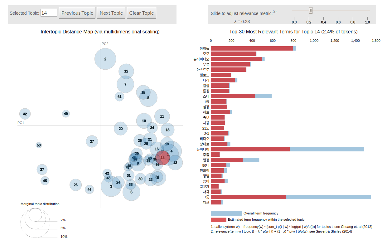
좌측은 topic vector 를 2 차원으로 축소하여 토픽 간의 관계를 살펴볼 수 있도록 도와줍니다. 비슷한 좌표를 지닌 토픽들은 비슷한 맥락을 지닙니다. 이를 위하여 LDAvis 는 토픽에서 단어가 발생할 확률 벡터인 \(P(w \vert t)\) 에 Principal Component Analysis (PCA) 를 적용하여 2 차원의 벡터로 압축합니다.
우측에는 각 토픽의 키워드가 제공됩니다. 키워드 점수 (relevance) 는 (1) 각 토픽에서 단어가 발생할 확률인 \(P(w \vert t)\) 와 (2) 이를 단어의 기본 발생 확률로 정규화한 \(\frac{P(w \vert t)}{P(w)}\) 가 \(\lambda\) 에 의하여 조합되어 계산됩니다. 사용자는 \(\lambda\) 를 조절하며 각 토픽에 주로 등장하는 단어와, 다른 단어와 차별성이 높은 단어들을 살펴볼 수 있습니다.
\[relevance(t,w) = \lambda \cdot P(w \vert t) + (1 - \lambda) \cdot \frac{P(w \vert t)}{P(w)}\]Python 라이브러리인 Gensim 을 이용하여 LDA 를 학습하였다면 아래와 같은 간단한 코드로 LDAvis 의 결과를 얻을 수 있습니다. 더 자세한 학습 코드는 이전의 pyLDAvis 포스트를 참고하세요.
from gensim.models import LdaModel
import pyLDAvis.gensim as gensimvis

lda_model = LdaModel(corpus, id2word=dictionary, num_topics=50)
prepared_data = gensimvis.prepare(lda_model, corpus, dictionary)
pyLDAvis.display(prepared_data)
k-means
k-means 는 다른 군집화 알고리즘과 비교하여 매우 적은 계산 비용을 요구하면서도 안정적인 성능을 보입니다. 그렇기 때문에 큰 규모의 데이터 군집화에 적합합니다. 문서 군집화의 경우에는 문서의 개수가 수만건에서 수천만건 정도 되는 경우가 많기 때문에 다른 알고리즘보다도 k-means 가 더 많이 선호됩니다. k-partition problem 은 데이터를 k 개의 겹치지 않은 부분데이터 (partition)로 분할하는 문제 입니다. 이 때 나뉘어지는 k 개의 partiton 에 대하여, “같은 partition 에 속한 데이터 간에는 서로 비슷하며, 서로 다른 partition 에 속한 데이터 간에는 이질적”이도록 만드는 것이 군집화라 생각할 수 있습니다. k-means problem 은 각 군집 (partition)의 평균 벡터와 각 군집에 속한 데이터 간의 거리 제곱의 합 (분산, variance)이 최소가 되는 partition 을 찾는 문제입니다.
\[\sum _{i=1}^{k}\sum _{\mathbf {x} \in S_{i}}\left\|\mathbf {x} -{\boldsymbol {\mu }}_{i}\right\|^{2}\]우리가 흔히 말하는 k-means 알고리즘은 Lloyd 에 의하여 제안되었습니다. 이는 다음의 순서로 이뤄져 있습니다.
- k 개의 군집 대표 벡터 (centroids) 를 데이터의 임의의 k 개의 점으로 선택합니다.
- 모든 점에 대하여 가장 가까운 centroid 를 찾아 cluster label 을 부여하고,
- 같은 cluster label 을 지닌 데이터들의 평균 벡터를 구하여 centroid 를 업데이트 합니다.
- Step 2 - 3 의 과정을 label 의 변화가 없을때까지 반복합니다.
우리가 list of str 형태의 문서 집합을 가지고 있을 때, scikit-learn 을 이용하여 k-means 를 학습하는 방법은 매우 간단합니다. 아래의 코드는 문서 집합을 bag-of-words model 로 표현한 다음 k-means 를 적용하는 과정까지의 코드입니다.
사실 문서 군집화를 위해서는 문서 간 거리를 Cosine 으로 정의하는 Spherical k-means 를 이용해야 합니다만, scikit-learn (<= 0.19.1) 에서는 이를 제공하지 않습니다. 오로직 Euclidean distance 만을 이용합니다. 그런데 Euclidean 은 벡터의 크기에 영향을 받습니다. 문서에 단어가 많을수록 term vector 의 크기 (norm) 는 커집니다. 이 문제를 해결하기 위한 임시 방편으로 L2 normalize 를 할 수 있습니다.
물론 bag-of-words model 에 L2 normalization 만을 적용한다고 Spherical k-means 가 되지는 않습니다. 이에 대한 이야기는 다른 포스트에서 설명하겠습니다. 여하튼, Euclidean distance 를 이용한 문서 군집화를 한다면 반드시 L2 normalization 을 해야 합니다.
from sklearn.feature_extraction.text import CountVectorizer
from sklearn.preprocessing import normalize
from sklearn.cluster import KMeans

docs = ['document format', 'list of str like']

# vectorizing
vectorizer = CountVectorizer()
X = vectorizer.fit_transform(docs)

# L2 normalizing
X = normalize(X, norm=2)

# training k-means
kmeans = KMeans(n_clusters=k).fit(X)

# trained labels and cluster centers
labels = kmeans.labels_
centers = kmeans.cluster_centers_
sklearn.cluster.KMeans 를 학습하면 labels_, cluster_centers_ 에 각 문서의 군집 레이블과 centroid vectors 가 저장되어 있습니다. 하지만 이 정보만을 가지고서 군집화 결과를 효과적으로 설명하기는 어렵습니다. 가장 좋은 설명은 그림이라 합니다. 이전 포스트에서 살펴보았던 pyLDAvis 를 이용하여 k-means 의 결과도 시각화 합니다.
k-means as Topic modeling
k-means 도 사실 토픽 모델링으로 이용 가능합니다. 실제로 LDA 와 같은 토픽 모델링과 k-means 와의 차이는 문서의 토픽 개수에 대한 가정입니다. LDA 는 한 문서에 여러 종류의 토픽이 존재할 수 있다 가정합니다. 하지만 k-means 는 하나의 문서가 하나의 토픽이라는 가정을 합니다. 이 가정은 오히려 어떤 문서 집합에서는 유용한 사전 지식 (prior) 이 됩니다. 주로 뉴스는 한 기사에 하나의 토픽이 있습니다. 반면 한 영화에 대한 여러 관점의 리뷰라면 여러 토픽이 섞여있을 수 있습니다. 우리가 한 문서에 하나의 토픽이 존재한다고 가정한다면 굳이 over-spec 인 LDA 를 이용할 필요는 없습니다.
또한 한 문서에 최대 두, 세개의 토픽이 균등히 섞일 수 있다고 가정한다면, 그리고 데이터의 양이 매우 많다면 k-means 를 LDA 의 대용으로 이용할 수도 있습니다. 대신에 이 경우에는 LDA 에서 기대하는 토픽의 개수가 10 개라면 k-means 에서는 100 ~ 500 개 수준으로 그 개수를 늘려야 합니다. 만약 실제 존재하는 토픽이 [\(0, 1, 2, \dots, 9\)] 라 할 때, 이들의 조합으로 [(\(0, 1\)), (\(0, 2\)), … ] 와 같은 토픽조합을 만들 수 있고 이들을 각각 하나의 군집으로 취급할 수 있기 때문입니다.
물론 이 때 적절한 토픽의 개수나 군집의 개수의 결정 문제가 따라오지만 이에 대해서는 일단 이야기 하지 않습니다. 이론상 k-means 를 토픽 모델링에 이용할 수 있다는 것 뿐입니다. 언제나 이론과 실제는 다르니까요 (실제로는 그냥 LDA 하나 학습하는 것도 잘 이뤄지지 않습니다).
Visualize k-means using pyLDAvis
이를 위해서는 pyLDAvis 의 함수를 뜯어볼 필요가 있습니다. 우리가 이용했던 pyLDAvis.gensim.prepare 함수는 gensim.models.LdaModel 의 parameters 로부터 필요한 정보를 추출한 뒤, pyLDAvis._prepare.prepare 함수에 넘겨줍니다. 이 함수에 입력되는 정보와 출력되는 정보를 살펴볼 필요가 있습니다.
pyLDAvis._prepare.prepare 함수
아래는 _prepare.prepare 함수의 argument 입니다. (topic, term) distribution, (doc, topic) distribution, doc length, vocab, term frequency 정보를 입력해야 합니다. 다른 값은 default 입니다. 이 값들은 이후에 다시 설명하겠습니다.
def prepare(topic_term_dists, doc_topic_dists, doc_lengths, vocab, term_frequency, \
            R=30, lambda_step=0.01, mds=js_PCoA, n_jobs=-1, \
            plot_opts={'xlab': 'PC1', 'ylab': 'PC2'}, sort_topics=True):
    ...
각 군집의 centroid 는 단어 크기의 벡터입니다. 각 element, centroid[c,w] 은 군집 \(c\) 에서 단어 \(w\) 가 얼마나 등장하였는지를 나타내는 weight 입니다. 만약 우리가 TF-IDF term weighting 을 이용하였다면 centroid[c,w] 는 군집 \(c\) 에서 단어 \(w\) 가 얼마나 중요한지를 나타낼 것입니다. 여하튼 centroid vector 의 각 elements 는 단어의 상대적인 중요도를 나타냅니다. 또한 non-negative 이기 때문에 이를 L1 normalization 을 하면 확률 분포로 이용할 수도 있습니다. 일단 topic_term_dists 를 대체할 정보는 찾았습니다.
앞서 살펴본 것처럼 k-means 는 문서에 하나의 토픽이 존재한다고 가정하는 토픽 모델링 입니다. 그렇기 때문에 doc_topic_dists 는 [0, 1, 0, …, 0] 과 같이 각 문서에 해당하는 label 에만 1 을 부여한 행렬로 대체할 수 있습니다.
문서의 길이 doc_lengths 는 bag-of-words model 로 만든 sparse matrix x 를 다음처럼 만들면 얻을 수 있습니다.
doc_lengths = x.sum(axis=1)그런데 이 형식이 numpy.ndarray 가 아니라 그 위의 abstract class 인 matrix 입니다. 이를 numpy.ndarray 의 column vector 로 변환하려면 다음과 같은 작업을 하여야 합니다.
import numpy as np

doc_lengths = np.asarray(x.sum(axis=1)).reshape(-1)
앞서 doc lengths 는 column sum 이었다면 term frequency 는 row sum 을 하면 됩니다.
import numpy as np

term_frequency = np.asarray(x.sum(axis=0)).reshape(-1)
vocab 이야 list of str 로, vectorizing 을 하는 과정에서 이미 얻었습니다. 이 재료를 _prepare.prepare 함수에 입력하여 PreparedData 를 얻을 수도 있습니다.
pyLDAvis.PreparedData
그런데 우리는 _prepare.prepare 함수에서 일어나는 일을 몇 개 변형하려 합니다. 직접 my_prepare 함수를 만들어 봅니다. 이를 위해서는 PreparedData 를 만들기 위해 필요한 데이터의 타입을 살펴봐야 합니다. init 함수의 첫 줄의 세 정보를 우리가 만들어야 합니다 (이 세 정보가 _prepare.prepare 함수가 만드는 정보입니다).
class PreparedData:
    def __init__(topic_coordinates, topic_info, token_table,
                 R, lambda_step, plot_opts, topic_order):
        ...
앞의 세 개의 arguments 인 topic_coordinates, topic_info, token_table 은 pandas.DataFrame 형식으로 저장된 테이블입니다. 즉 csv 형식으로 저장할 수 있는 정보입니다. 그러므로 이 포스트에서는 csv 테이블로 세 정보를 설명합니다.
솔직히 LDAvis 가 이용하는 세 종류 table 의 naming 이나 각 table 의 column name 이 직관적이지 않고, 잘 정리된 형태도 아닙니다. 하지만 Java Script 를 이용하여 밑바닥부터 시각화 작업을 하는 것보다 만들어져 있는 LDAvis 를 이용하여 k-means 를 시각화 하는 것이 더 빠를테니 도전해 봅시다!
topic coordinates
topic coordinates 는 HTML 의 왼쪽에 위치한 topic vector 의 2 차원 좌표입니다. 이들은 각각 x, y 로 표시됩니다. topics 는 1 부터 num topics 까지 idx 를 증가하는 것이며, cluster 는 1 로 일괄되게 저장합니다. Freq 는 토픽을 표현하는 원의 지름 입니다. 이 크기가 클수록 자주 등장한 토픽이라는 의미이며, 이는 \(P(t)\) 의 값에 비례하여 만듭니다.
| topic | x | y | topics | cluster | Freq |
|---|---|---|---|---|---|
| 50 | -0.746 | -2.666 | 1 | 1 | 3.510 |
| 4 | 2.837 | -2.585 | 2 | 1 | 3.134 |
| 54 | 1.428 | 1.844 | 3 | 1 | 2.442 |
| 85 | 0.488 | -4.691 | 4 | 1 | 2.260 |
| 38 | -0.409 | -1.471 | 5 | 1 | 2.253 |
| 9 | 0.597 | -3.140 | 6 | 1 | 2.157 |
| 13 | -2.184 | -1.300 | 7 | 1 | 2.126 |
topic info
topic info 는 조금 복잡합니다. pyLDAvis 에서 term 은 단어의 idx 입니다. 대문자로 시작하는 Term 은 단어의 실제 str 값입니다. (term, Category) 는 topic info 테이블의 key 입니다. Category 는 각 row 가 어떤 토픽에 해당하는지를 저장합니다. Default 는 어떤 토픽도 선택하지 않았을 때입니다. Freq 는 term 이 Category 에 등장한 횟수이며, 추정값입니다. Total 은 문서 전체에서의 term frequency 입니다. loglift 는 \(log \frac{P(w \vert t)}{P(w)}\) 이며, distriminative power 를 표현하는 값입니다. logprob 는 \(log P(w \vert t)\) 이며, 단어 \(w\) 가 토픽 \(t\) 에 얼만큼 등장하는지 coverage 를 보여주는 값입니다.
| term | Category | Freq | Term | Total | loglift | logprob |
|---|---|---|---|---|---|---|
| 1985 | Default | 0.99 | 기자 | 27189 | 25.000 | 25.000 |
| 3424 | Default | 0.99 | 무단 | 21575 | 21.902 | 21.902 |
| 337 | Default | 0.99 | 20일 | 20858 | 21.507 | 21.507 |
| … | … | … | … | … | … | … |
| 2434 | Topic1 | 2550 | 뉴시스 | 9950 | 5.324 | -5.489 |
| 2681 | Topic1 | 3731 | 대한 | 9054 | 4.995 | -3.277 |
| 304 | Topic2 | 1523 | 2016 | 11149 | 6.150 | -5.320 |
| 1121 | Topic2 | 995 | 것으로 | 10447 | 5.763 | -4.615 |
token table
token table 은 각 term 이 특정 topic 에 등장한 비율입니다. 즉 한 단어에 대하여 모든 row 의 Freq 의 합은 1 이하입니다. 이름이 topic term proportion 이면 더 좋았을 것 같네요.
| term | Topic | Freq | Term |
|---|---|---|---|
| 4697 | 1 | 0.299 | 선언 |
| 962 | 1 | 0.546 | 강진 |
| 2667 | 1 | 0.074 | 대표 |
| 4950 | 1 | 0.209 | 손학규 |
| 7448 | 1 | 0.223 | 정계복귀 |
| 7447 | 1 | 0.439 | 정계 |
| 6566 | 1 | 0.603 | 은퇴 |
| 3849 | 1 | 0.840 | 백련사 |
우리는 loglift, logprob 의 값과 topic coordinate (x, y) 를 만들어야 합니다. token table 의 Freq (topic term proportion) 은 상대적으로 만들기 쉽습니다. topic_order 는 topic coordinates 의 row 순서대로의 topic idx 입니다. 길이가 n_topics 인 list of int 입니다.
Making topic coordinates
우리는 k-means 를 이용하여 학습한 centroid 와 labels 를 이용하여 LDAvis 에 입력할 정보들을 만듭니다.
LDAvis 는 PCA 를 이용하여 2 차원 벡터를 학습합니다. 하지만 bag-of-words model 처럼 sparse vector 로 표현되는 고차원 벡터간 거리는 Cosine distance 를 이용하는 것이 좋습니다. 그리고 원 공간에서 비슷한 점들은 2 차원에서도 비슷해야 원 공간을 이해하기가 좋습니다. 즉 locality 정보가 중요합니다. 하지만 PCA 는 global variance 정보에 집중합니다. 그러므로 PCA 대신 t-SNE 를 이용합니다. 이 값을 이용하여 centroid vector 를 2 차원으로 압축합니다. scikit-learn 의 0.19.1 이후부터는 t-SNE 의 metric 을 ‘cosine’ 으로 설정할 수 있습니다. 각 좌표의 값을 [-5, 5] 사이가 되도록 scaling 도 합니다.
coordinates = TSNE(n_components=2, metric='cosine').fit_transform(centers)
coordinates = 5 * coordinates / max(coordinates.max(), abs(coordinates.min()))
cluster size 는 labels 을 카운팅함으로써 확인할 수 있습니다. 이 값의 root 에 비례하여 cluster size 를 만듭니다. 크기가 가장 작은 cluster 는 0.2 의 Freq 값을, 그리고 가장 큰 cluster 의 Freq 는 radious + 0.2 가 되도록 scaling 도 합니다.
cluster_size = np.asarray(
    [np.sqrt(cluster_size[c] + 1) for c in range(n_clusters)])
cs_min, cs_max = cluster_size.min(), cluster_size.max()
cluster_size = radius * (cluster_size - cs_min) / (cs_max - cs_min) + 0.2
위 내용을 정리하면 아래와 같습니다.
from collections import Counter
from collections import namedtuple
from sklearn.manifold import TSNE
import numpy as np

TopicCoordinates = namedtuple('TopicCoordinates', 'topic x y topics cluster Freq'.split())

cluster_size = Counter(labels)
cluster_size = np.asarray([cluster_size.get(c, 0) for c in range(n_clusters)])

def _get_topic_coordinates(centers, cluster_size, radius=5):
    n_clusters = centers.shape[0]
    coordinates = TSNE(n_components=2, metric='cosine').fit_transform(centers)
    coordinates = 5 * coordinates / max(coordinates.max(), abs(coordinates.min()))

    cluster_size = np.asarray(
        [np.sqrt(cluster_size[c] + 1) for c in range(n_clusters)])
    cs_min, cs_max = cluster_size.min(), cluster_size.max()
    cluster_size = radius * (cluster_size - cs_min) / (cs_max - cs_min) + 0.2

    topic_coordinates = [
        TopicCoordinates(c+1, coordinates[i,0], coordinates[i,1], i+1, 1, cluster_size[c])
        for i, c in enumerate(sorted(range(n_clusters), key=lambda x:-cluster_size[x]))
    ]

    topic_coordinates = sorted(topic_coordinates, key=lambda x:-x.Freq)
    return topic_coordinates
Making keyword score
loglift 와 logprob 는 keyword score 에 해당합니다. 이전 포스트에서 군집화의 키워드를 정의하는 방법을 이야기하였습니다. 간단히 요약하면 아래와 같습니다.
우리는 cluster center vectors 를 이용하여 salient and discriminative 한 키워드 집합을 선택합니다. Salient terms 는 각 군집의 center 벡터에서 큰 weight 를 지닌 단어입니다. 다음으로 우리가 해야 할 작업은 discriminative power 를 수식으로 정의하는 것입니다. Discriminative power 가 큰 단어는 해당 군집에서는 자주 등장하지만, 다른 군집에서는 등장하지 않은 단어입니다. 즉, 유독 weight 가 큰 단어입니다. 이를 다음과 같은 수식으로 정의합니다. \(c\) 는 군집이며 \(v\) 는 단어입니다. $w(v, c)\(는 단어\)v\(의 군집\)c$$ 에서의 weight 입니다.
\[s(v, c) = \frac{w(v \vert c)}{w(v \vert c) + w(v \vert \tilde{c})}\]- \(w(v \vert c)\) : 군집 c 의 center vector 에서의 term v 에 대한 weight
- \(w(v \vert \tilde{c})\) : 군집 c 를 제외한 다른 문서 집합들에서의 term v 에 대한 weight
loglift 는 discriminative power 에 관련된 항목입니다. 이 값으로 \(\frac{w(v \vert c)}{w(v \vert c) + w(v \vert \tilde{c})}\) 를 이용합니다. Coverage 에 해당하는 logprob 로 \(w(v \vert c)\) 를 이용합니다.
for c, n_docs in enumerate(cluster_size):
    topic_idx = c + 1
    n_prop = l1_normalize(weighted_center_sum - (centers[c] * n_docs))
    p_prop = l1_normalize(centers[c])
    indices = np.where(p_prop > 0)[0]
    ...
각 클러스터마다 크기가 다르기 때문에 클러스터의 크기를 곱한 weighted_centers 를 만듭니다. 이 값을 이용하여 \(w(v \vert c)\) 인 p_prop 와 \(w(v \vert \tilde{c})\) 인 n_prop 를 만듭니다. loglift 는 p_prop / (n_prop + p_prop) 로 정의합니다. p_prop 가 큰 각 클러스터마다 n_candidate_words 개의 단어에 대하여 loglift 와 logprob 에 해당하는 값을 계산하여 scores 로 만듭니다.
for c, n_docs in enumerate(cluster_size):
    ...
    indices = sorted(indices, key=lambda idx:-p_prop[idx])[:n_candidate_words]
    scores = [(idx, p_prop[idx] / (p_prop[idx] + n_prop[idx])) for idx in indices]
각 클러스터에 대해서는 loglift 와 logprob 의 값을 만들어줘야 하지만, Default Category 를 위해서는 most frequent term 만 선택하면 됩니다. 이는 term_frequency.argsort()[::-1] 를 이용하여 찾을 수 있습니다. 빈도수가 큰 n_candidate_words 에 대하여 term frequency 에 비례하는 loglift, logprob 의 값을 만들어줍니다. Scale 은 임의로 [10, 25] 로 정의하였습니다.
default_terms = term_frequency.argsort()[::-1][:n_candidate_words]
default_term_frequency = term_frequency[default_terms]
default_term_loglift = 15 * default_term_frequency / default_term_frequency.max() + 10
for term, freq, loglift in zip(default_terms, default_term_frequency, default_term_loglift):
    ...
위 내용을 정리하면 아래와 같습니다.
weighted_centers = np.zeros((n_clusters, n_terms))
for c, n_docs in enumerate(cluster_size):
    weighted_centers[c] = centers[c] * n_docs

TopicInfo = namedtuple('TopicInfo', 'term Category Freq Term Total loglift logprob'.split())

def _get_topic_info(centers, cluster_size, index2word,
    weighted_centers, term_frequency, n_candidate_words=100):

    l1_normalize = lambda x:x/x.sum()
    n_clusters, n_terms = centers.shape

    weighted_center_sum = weighted_centers.sum(axis=0)
    total_sum = weighted_center_sum.sum()
    term_proportion = weighted_centers / weighted_center_sum

    topic_info = []

    # Category: Default
    default_terms = term_frequency.argsort()[::-1][:n_candidate_words]
    default_term_frequency = term_frequency[default_terms]
    default_term_loglift = 15 * default_term_frequency / default_term_frequency.max() + 10
    for term, freq, loglift in zip(default_terms, default_term_frequency, default_term_loglift):
        topic_info.append(
            TopicInfo(
                term,
                'Default',
                0.99,
                index2word[term],
                term_frequency[term],
                loglift,
                loglift
            )
        )

    # Category: for each topic
    for c, n_docs in enumerate(cluster_size):
        if n_docs == 0:
            keywords.append([])
            continue

        topic_idx = c + 1

        n_prop = l1_normalize(weighted_center_sum - (centers[c] * n_docs))
        p_prop = l1_normalize(centers[c])

        indices = np.where(p_prop > 0)[0]
        indices = sorted(indices, key=lambda idx:-p_prop[idx])[:n_candidate_words]
        scores = [(idx, p_prop[idx] / (p_prop[idx] + n_prop[idx])) for idx in indices]

        for term, loglift in scores:
            topic_info.append(
                TopicInfo(
                    term,
                    'Topic%d' % topic_idx,
                    term_proportion[c, term] * term_frequency[term],
                    index2word[term],
                    term_frequency[term],
                    loglift,
                    p_prop[term]
                )
            )

    return topic_info
Making token table
만들어둔 topic info 를 이용하면 손쉽게 token table 을 만들 수 있습니다. weighted_centers 의 row sum 으로 weighted_centers 를 나누면 각 클러스터 \(c\) 마다 단어 \(w\) 가 전체 중에서 얼마나 등장하였는지 그 비율이 계산됩니다.
term_proportion = weighted_centers / weighted_centers.sum(axis=0)이를 이용하여 topic info 에 입력된 단어들에 대해서만 따로 token table 을 만들어줍니다.
TokenTable = namedtuple('TokenTable', 'term Topic Freq Term'.split())

def _get_token_table(weighted_centers, topic_info, index2word):
    term_proportion = weighted_centers / weighted_centers.sum(axis=0)

    token_table = []
    for info in topic_info:
        try:
            c = int(info.Category[5:])
        except:
            # Category: Default
            continue
        token_table.append(
            TokenTable(
                info.term,
                c,
                term_proportion[c-1,info.term],
                info.Term
            )
        )

    return token_table
Making my_prepare
세 종류의 테이블을 만들 함수는 준비했습니다. 이제 데이터를 입력받아 세 테이블을 만드는 kmeans_to_prepared_data 함수를 만듭니다.
이 함수의 입력값은 bow model, index 2 word, centroid vector, labels, 이며, setting 을 위한 값들도 입력받습니다. 각각의 정보는 아래와 같습니다.
| Parameter | default | note |
|---|---|---|
| bow | . | sparse matrix, scipy.sparse.csr_matrix |
| index2word | . | list of str |
| centers | . | numpy.ndarray |
| labels | . | 군집 레이블, numpy.ndarray or list of int |
| radious | 3.5 | 원의 크기의 최대값 |
| n_candidate_words | 50 | keyword 로 선정될 가능성이 있는 후보 단어의 개수 (n_printed_words 보다 크거나 같아야 함) |
| n_printed_words | 30 | HTML 우측에 출력되는 단어의 개수 |
| lambda_step | 0.01 | \(\lambda\) 값을 조절할 때의 step size |
| plot_opts | {‘xlab’: ‘t-SNE1’, ‘ylab’: ‘t-SNE2’}) | x, y 좌표축에 입력될 이름 |
위 값들을 입력받아 topic coordinates, token table, topic info 테이블을 만들고, 이를 LDAvis.PreparedData 의 입력 형식인 pandas.DataFrame 으로 변환하여 줍니다. topic oder 는 cluster_size 의 argsort 값을 역순으로 정렬하여 list 로 만들어줍니다. 그 뒤 PreparedData 에 이 값들을 입력합니다.
def kmeans_to_prepared_data(bow, index2word, centers, labels, radius=3.5,
    n_candidate_words=50, n_printed_words=30, lambda_step=0.01,
    plot_opts={'xlab': 't-SNE1', 'ylab': 't-SNE2'}):

    n_clusters = centers.shape[0]
    n_docs, n_terms = bow.shape

    cluster_size = Counter(labels)
    cluster_size = np.asarray([cluster_size.get(c, 0) for c in range(n_clusters)])

    term_frequency = np.asarray(bow.sum(axis=0)).reshape(-1)
    term_frequency[np.where(term_frequency == 0)[0]] = 0.01

    weighted_centers = np.zeros((n_clusters, n_terms))
    for c, n_docs in enumerate(cluster_size):
        weighted_centers[c] = centers[c] * n_docs

    # prepare parameters
    topic_coordinates = _get_topic_coordinates(
        centers, cluster_size, radius)

    topic_info = _get_topic_info(
        centers, cluster_size, index2word,
        weighted_centers, term_frequency, n_candidate_words)

    token_table = _get_token_table(
        weighted_centers, topic_info, index2word)

    topic_order = cluster_size.argsort()[::-1].tolist()

    # convert to pandas.DataFrame
    topic_coordinate_df = _df_topic_coordinate(topic_coordinates)
    topic_info_df = _df_topic_info(topic_info)
    token_table_df = _df_token_table(token_table)

    # ready pyLDAvis.PreparedData
    prepared_data = pyLDAvis.PreparedData(
        topic_coordinate_df,
        topic_info_df,
        token_table_df,
        n_printed_words,
        lambda_step,
        plot_opts,
        topic_order
    )

    # return
    return prepared_data
Demo
2016-10-20 뉴스 30,091 건에 대하여 명사를 추출한 다음 k=100 으로 설정하여 k-means 를 학습하였습니다. 그 뒤 위 함수를 이용하여 PreparedData 를 만들고 display 를 하였습니다.
위 코드들은 깃헙, https://github.com/lovit/kmeans_to_pyLDAvis 에 올려두었습니다.
import pyLDAvis
from kmeans_visualizer import kmeans_to_prepared_data

prepared_data = kmeans_to_prepared_data(x, index2word, centers, labels)
pyLDAvis.display(prepared_data)
말이 되지 않는 군집들이 존재하기도 합니다. 이들을 걸러내는 것은 k-means 같은 문서 군집화 알고리즘의 역할입니다. 이부분은 일단 넘어갑시다 (문서 군집화의 성능 향상은 따로 다뤄야할 어려운 문제입니다). \(\lambda\) 를 조절함으로써 군집에 많이 나오는 단어와 다른 군집과 구분이 되는 단어를 살펴볼 수 있습니다. 그리고 비슷한 2 차원 좌표를 지닌 군집들은 비슷한 키워드를 지니고 있음도 볼 수 있습니다.
사실 LDA 대신 k-means 를 이용할 때에는 k 를 훨씬 크게 잡아주고 비슷한 군집을 하나의 군집으로 묶어주는 후처리 과정도 필요합니다. 이에 대해서는 이번 포스트에서 다루지 않았습니다. 하지만, 더 이상 군집화 결과를 군집 레이블의 리스트로 보지 않아도 됩니다.
Reference
- Buchta, C., Kober, M., Feinerer, I., & Hornik, K. (2012). Spherical k-means clustering. Journal of Statistical Software, 50(10), 1-22.